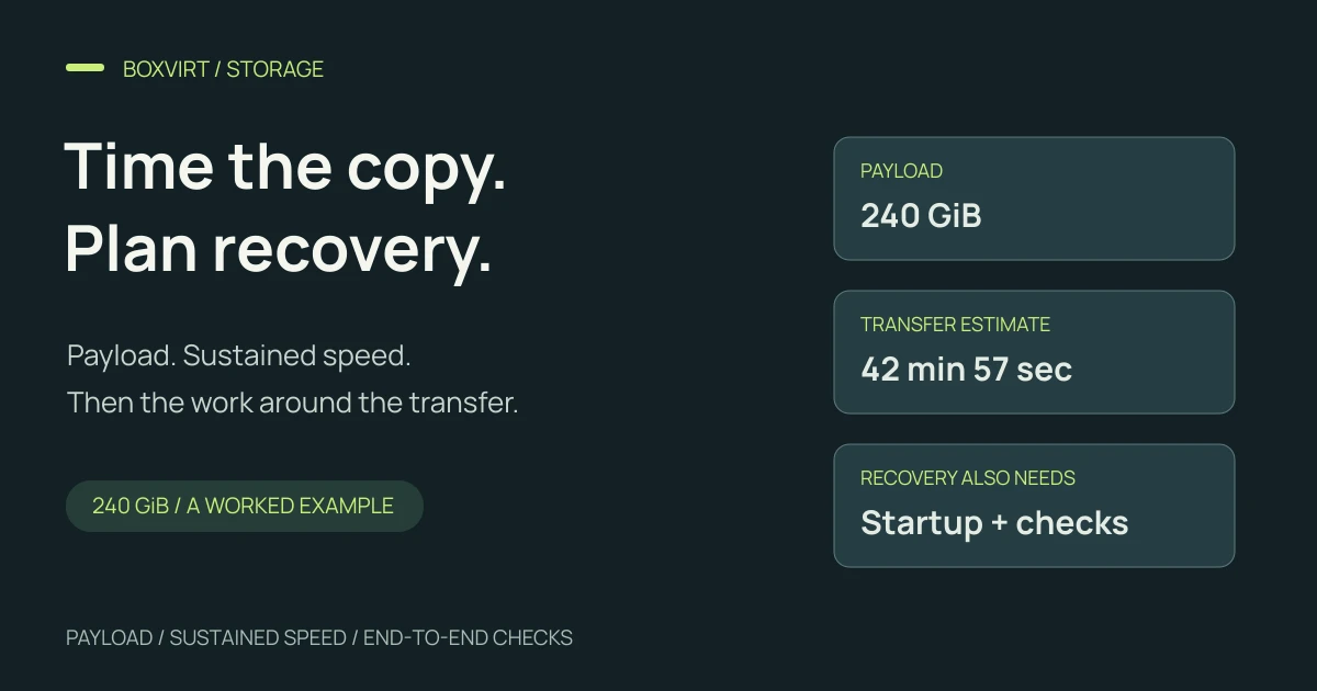
Transferring 240 GiB over a 1 Gbps connection at an assumed 80% payload efficiency takes about 42 minutes 57 seconds. That estimates one transfer phase. Getting the application back also requires access to the backup, usable destination storage, startup and a check that the recovered service works.
For a useful estimate, identify the bytes that will cross the connection, choose a rate that applies to that path, and give the transfer its own window inside the recovery plan. We will calculate both the duration and the speed needed for a target window. All sizes, rates and time budgets below are illustrative inputs, not measurements of Boxvirt’s infrastructure.
Choose the payload for the operation you are planning
The provisioned size of a VM disk, the amount of data stored in a backup repository and the bytes transmitted by one job can be different. Write down which operation you mean before using a size:
| Operation | Size to investigate |
|---|---|
| First backup to a destination | Data the backup client needs to transmit for that initial operation |
| Later incremental backup | Data transmitted after that backup system’s reuse and reduction |
| Copy of an archive file | The actual archive size, if that file is what crosses the connection |
| Recovery of a guest or application | Data fetched for the selected recovery, which can differ from the latest backup’s upload |
For example, the Proxmox Backup technical overview explains how snapshots reference chunks and later uploads can reuse chunks already present on the server. A small incremental upload therefore does not tell you the payload needed to recover the whole selected snapshot.
Use logs from a comparable operation where available. Keep logical data size, transmitted payload and destination writes labelled separately. Compression, deduplication and sparse storage can change their relationship; this calculation does not predict those savings.
Keep data units and rate units visible
The NIST binary-prefix reference defines a GiB as 1,073,741,824 bytes and a GB as 1,000,000,000 bytes. A byte contains eight bits. Here, Mbps means one million bits per second, while MB/s means one million bytes per second.
240 GiB = 240 × 1,073,741,824 = 257,698,037,760 bytes
1 Gbps = 1,000 Mbps = 1,000,000,000 bits/second
100 MB/s = 800 Mbps
Changing 240 GiB to 240 GB changes the amount of data. It is not just a different display label. Likewise, entering 100 MB/s as 100 Mbps makes the assumed rate eight times smaller.
Calculate the transfer phase
For an assumed connection rate and a chosen payload-efficiency factor:
Transfer seconds = payload bytes × 8 ÷ (connection bits/second × efficiency)
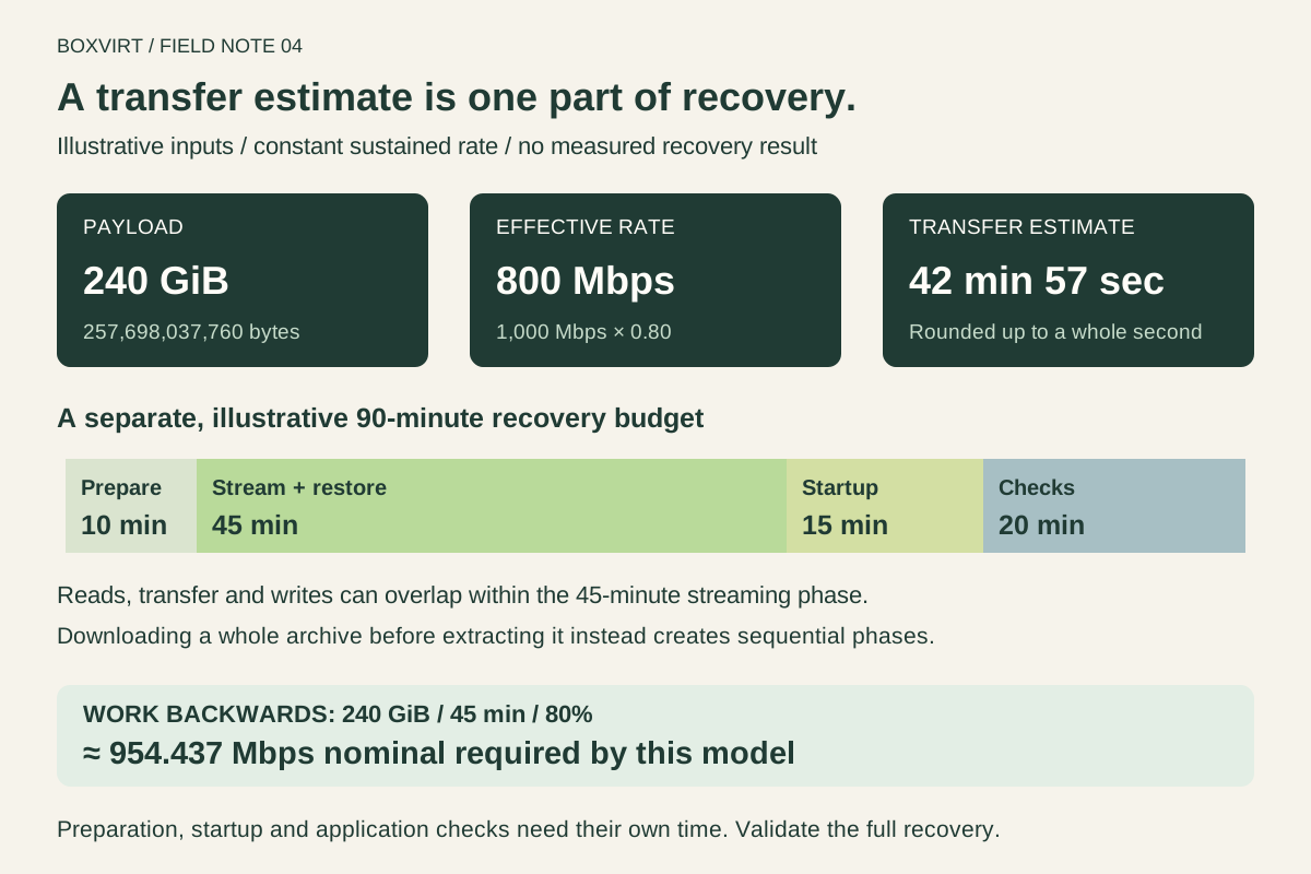
Efficiency is a fraction in the formula. In our example, 80% becomes 0.8, so the effective payload rate is 800 Mbps, or 100 MB/s:
Seconds = 257,698,037,760 × 8 ÷ (1,000,000,000 × 0.8)
        = 2,576.9803776
Rounded up to a whole second, that is 42 minutes 57 seconds. The 80% factor is a scenario input. It is not a claim about typical Ethernet efficiency or the performance of your backup system.
These three scenarios show the effects of changing the inputs:
| Payload | Assumed connection | Efficiency | Estimated transfer duration |
|---|---|---|---|
| 240 GiB | 1,000 Mbps | 80% | 42 min 57 sec |
| 240 GB | 1,000 Mbps | 80% | 40 min |
| 240 GiB | 250 Mbps | 80% | 2 hr 51 min 48 sec |
To reproduce the first row in the download and upload time calculator, choose Transfer time, enter 240 GiB, 1,000 Mbps and 80%. The displayed duration rounds up, while the calculation retains the fractional seconds. The same arithmetic works for backup uploads and restore downloads; their payloads and available rates must be chosen independently.
Use an observed payload rate without discounting it again
Suppose a comparable copy averages an illustrative 80 MiB/s over the transfer phase. That is already an observed payload rate. Enter 80 MiB/s and 100% efficiency when modelling the same phase, rather than applying another allowance for overhead that the observation already includes.
For 240 GiB:
Seconds = 240 × 1,024 MiB ÷ 80 MiB/second
        = 3,072 seconds = 51 minutes 12 seconds
Applying an extra 80% factor would instead produce 64 minutes. That is a different, deliberately reduced-rate scenario; it should not be presented as the unchanged measured-rate estimate.
Check that the observation is an average, not a brief peak, and that its bytes and elapsed time refer to the operation you are estimating. The upload side of a remote connection may also have a different limit from the download side. Shared traffic, remote throttling, source reads and destination writes can all constrain sustained progress.
Give transfer a window inside the recovery objective
A recovery-time objective applies to recovery of the service or system, not merely the end of a file copy. See the NIST recovery-time objective definition for the broader recovery context.
Consider this hypothetical 90-minute planning budget:
| Phase | Chosen allowance | What must be included |
|---|---|---|
| Prepare and obtain access | 10 min | Find the backup, credentials and keys; prepare the target |
| Stream data and restore to storage | 45 min | Fetch, process and write data along the restore path |
| Start the guest and application | 15 min | Boot and satisfy required service dependencies |
| Validate the recovered service | 20 min | Check expected data and a real application operation |
| Total | 90 min | End-to-end budget, not a measured recovery result |
The transfer calculation must fit the 45-minute data phase, rather than using all 90 minutes. Our 42 min 57 sec network estimate leaves only about 2 min 3 sec of that phase. Source processing or slow writes could use that margin or become the limiting part of the phase themselves.
Reads, transfer and writes often overlap in a streaming restore. Measure or model that combined path; do not automatically add three full-duration passes over the same data. If your workflow downloads an archive completely and then extracts it as a separate step, those sequential phases need separate time. Compressed input bytes and expanded destination bytes also require a consistent basis before comparing their rates.
The budget above is an example of how to organise the estimate. It does not establish that a real application can recover in 90 minutes.
Work backwards to the required connection speed
For 240 GiB within a 45-minute transfer window at the same assumed 80% factor:
Connection bits/second = payload bytes × 8 ÷ (target seconds × efficiency)
Required Mbps = 257,698,037,760 × 8 ÷ (2,700 × 0.8) ÷ 1,000,000
              ≈ 954.437 Mbps
In the transfer calculator, choose Required connection speed, enter 240 GiB, 45 minutes and 80%. The result is approximately 954.437 Mbps, before any additional contingency. This is the model’s required nominal rate; the effective payload rate is about 763.550 Mbps. It is not a guaranteed service requirement from a provider.
A faster advertised connection helps only if the rest of the recovery path can sustain the corresponding progress. When testing a local restoration, Internet bandwidth might not be part of the path at all.
Replace assumptions with a repeatable recovery record
For the next planned restore test, record the backup identity, requested scope, units and payload; source and target; phase timestamps; sustained rates; concurrent workload; and the application check that marks completion. Keep successful data transfer distinct from successful application recovery.
The Proxmox Backup client documentation recommends periodic recovery tests. It also describes benchmarks for compression, encryption and, when a repository is supplied, TLS upload speed. Such a benchmark can help investigate one part of the path, while a timed application recovery checks the complete sequence.
If a run misses the budget, identify which phase exceeded its allowance before changing the link estimate. A log showing slow source reads calls for a different investigation from a long wait for a key or an application that will not start. Use the Proxmox backup and restore checklist for the recovery workflow, and the ZFS capacity planning guide when checking space on the destination. Transfer time and destination capacity need to work together in the final plan.